Introduction to Theory, Practice of Radioligand Binding

Radioactivity, Radioligands and Binding Assays

As we discussed, a radioligand is a radioactively labeled drug that can associate with a receptor, transporter, enzyme, or any protein of interest. Measuring the rate and extent of binding provides information on the number of binding sites, and their affinity and pharmacological (biological) characteristics.

There are three commonly used experimental protocols:

Saturation binding experiments. These are the experiments whose theoretical basis we just derived. In these experiments the extent of binding is measured in the presence of different concentrations of the radioligand. From an analysis of the relationship between binding and ligand concentration, we can determine the number of binding sites, B_max, and ligand affinity, K_D.
Kinetic experiments. Saturation and competition experiments are allowed to incubate until binding has reached equilibrium. Kinetic experiments measure the time course of binding and dissociation to determine the rate constants for radioligand binding and dissociation. Together, these values also permit a calculation of the K_D.
Competitive binding experiments. Measure the binding of a single concentration of radioligand at various concentrations of an unlabeled competitor. Analyze these data to learn the affinity of the receptor for the competitor.

How to Separate Bound from Free

For any of these approaches to work, one must be able to determine how much radioligand is associated with the receptor, and how much is unbound. It is fortunate that the huge majority of target macromolecules are either insoluble (e.g., membranous) or can be made insoluble with simple biochemical tricks (e.g., using polyethylene glycol). There are three general approaches of which you should be aware.

Equilibrium dialysis

Technical problems prevent its use except in rare circumstances. Some issues include: degradation or sticking of receptor or ligand; cumbersome nature of assays when large numbers of samples are needed; time to obtain equilibrium; etc. Moreover, this technique cannot be used for kinetic analysis.

Centrifugation:

The [R] changes during pelleting and trapped radioactivity increases non-specific binding (NSB; see later sections). One can calculate time allowable for separation based on K_D and the derived rate constants; the relationship will be logarithmic. The table to the left makes the assumption that separation must be complete in ca. 0.15 t_0.5 if one is to avoid losing more than 10% of DR complex, thus introducing unacceptable error. As one can see, assays with low affinity ligands introduce very specific experimental problems.

K_D (nM)

1000

100

0.1

0.15(t_0.5) (sec)

0.1

10.

100.

1000.

Filtration:

With sufficiently high K_D, several washes allow very low NSB. Cold wash buffer (like a cold centrifuge above) will increase further the separation time [see values for centrifugation (above)].

Total vs. free concentrations of ligand. Ligand depletion.

The equations that describe the law of mass action include the variable F ([Ligand]), the free radioligand. In many experimental situations, you can assume that only a very small fraction of the ligand ever binds to receptors. In these situations, you can assume that the free concentration of ligand is approximately equal to the concentration you added. This assumption vastly simplifies the analysis of binding experiments, and the standard analysis methods depend on this assumption. In other situations, a large fraction of the ligand binds to the receptors. This means that the concentration of ligand free in solution does not equal the concentration you added, and the discrepancy is not the same in all tubes or at all times. The free ligand concentration is depleted by binding. Many investigators use this rule of thumb. If less than 10% of the ligand binds to receptors, don't worry about ligand depletion. If more than 10% of the ligand binds, you have three choices:

Change the experimental conditions. The simplest approach is to decrease the amount of receptor in the incubation by using less tissue or fewer cells. The problem is that this will decrease the number of radioactive counts. The way around this is to increase the reaction volume without changing the amount of tissue. The problem with this approach is that it requires more radioligand, which is usually very expensive.
Measure the free concentration of ligand in every tube. This is fairly straightforward if you use centrifugation or equilibrium dialysis, but is difficult if you use vacuum filtration. One can also estimate the free concentration by subtracting the total bound from the total added.
Use analysis techniques that adjust for the difference between the concentration of added ligand and the concentration of free ligand.

Radioactivity

Specific Radioactivity

When you buy radioligands, the packaging usually states the specific radioactivity as Curies per millimole (Ci/mmol). Since you measure counts per minute (cpm) , the specific radioactivity is more useful when stated in terms of cpm. Often the specific radioactivity is expressed as cpm/fmol (1 fmol = 10^-15 mole). To convert from Ci/mol to cpm/fmol, you need to know the efficiency of your counter. Efficiency is the fraction of the radioactive disintegration that are detected by the counter.

Radionuclides that decay with high energy can be counted more efficiently than those with low energies modes. For example, ¹²⁵I can be counted at very high efficiencies, usually 70-90+% depending on the geometry of the gamma counter (e.g., if the detector doesn’t entirely surround the tube, some gamma rays miss the detector).

With ³H, the efficiency of counting is much lower (maximally ca. 60%). The low efficiency is mostly a consequence of the physics of decay, and can not be improved by better instrumentation. When a tritium atom decays, a neutron converts to a proton and the reaction shoots off an electron and neutrino. The energy released is always the same, but it is randomly partitioned between the neutrino (not detected) and an electron (that we try to detect). When the electron has sufficient energy, it will travel far enough to encounter a fluor molecule in the scintillation fluid. This fluid amplifies the signal and gives off a flash of light detected by the scintillation counter. The intensity of the flash (number of photons) is proportional to the energy of the electron. If the electron has insufficient energy, it is not captured by the fluor and is not detected. If it has low energy, it is captured but the light flash has few photons and is not detected by the instrument. Since the decay of many tritium atoms does not lead to a detectable number of photons, the efficiency of counting is less than 100%.

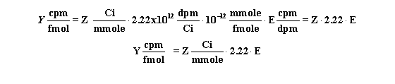
To convert from Ci/mmol to cpm/fmol, you need to know that 1 Ci equals 2.22 x 10¹² dpm (disintegrations per minute). Another unit of radioactivity that is becoming more common is the Becquerel (Bq). 1 mCi = 27.0270 MBq (that’s mega, not milli). The same exercise applies if you receive your radioactive sample in units of Bq.

Use this equation to convert Z Ci/mmol to Y cpm/fmol when the counter has an efficiency (expressed as a fraction) equal to E.

Calculating the concentration of the radioligand

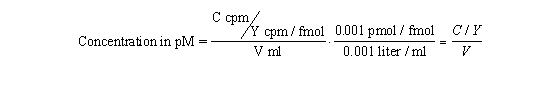
Rather than trust your dilutions, you can accurately calculate the concentration of radioligand in a stock solution. Measure the number of counts per minute in a small volume of solution and use this equation. C is cpm counted, V is volume of the solution you counted in ml, and Y is the specific activity of the radioligand in cpm/fmol (calculated in the previous section).

Radioactive decay

Radioactive decay is entirely random. A particular atom has no idea how old it is, and can decay at any time. The probability of decay at any particular interval is the same as the probability of decay at any other interval. If you start with N₀ radioactive molecules, the number remaining at time t is:

K_Decay is the rate constant of decay expressed in units of inverse time. Each radioactive isotope has a different value of K_Decay. The half-life (t_½) is the time it takes for half the isotope to decay. Half-life and decay rate constant are related by this equation:

It is this relationship that allowed us to formulate the equation presented earlier (and shown below) that uses the t_0.5 rather than the less commonly seen K_decay.

Selecting the radioligand

What chemical structure: agonist vs. antagonist

In general antagonists are used much more widely, in large measure because they often have much higher affinity than available agonists. (Discussion: why is this?) Resulting technical problems (degradation or sticking of receptor or ligand; cumbersome nature of assays when large numbers of samples are need; time to obtain equilibrium; etc.) have limited use of agonists with most receptors.

Choice of isotope

One can predict what type of radionuclide can be used successfully based on the density of receptors in the preparation being studied. This is either known from direct experimental evidence, or can be estimated by analogy to well characterized systems. Usually, one finds densities of from 10-500 fmol receptor/mg protein in "normal neural tissue", and from 200-3,000 fmol/mg in transfected cells, depending on the promoter used and other factors.

One can decide what radionuclides are suitable based on the estimated density of receptors and on elementary principles of detection of radioactivity. These calculations needed to determine feasibility for use of a radioligand in radioreceptor assays are identical to those for the use of radioisotopes in any biology problem. If you are not familiar with such calculations, please ask in class or see me before class.

The factors to consider include:

environmental and experimental background
efficiency of counting
amount of radiolabel incorporation into radioligand
specific activity of radionuclide

The specific activity of the radionuclide is based solely on its half-life, and is independent on the mode or energy of decay. The following table shows the half-lives for commonly used radioisotopes. The table also shows the specific activity assuming that each molecule is labeled with one atom of an isotope (as is often the case with ¹²⁵I and ³²P). Tritiated molecules often incorporate several tritium atoms, resulting in increased the specific radioactivity of the molecule.

Radionuclide	Half life	Specific Activity (Ci/mmol)	Decays to:	b Energy (keV)
³H	12.43 y	28.8	³He	18
¹²⁵I	59.6 d	2176	¹²⁵Te	-
³²P	14.3 d	9131	³²S	1710
³⁵S	87.4 d	1494	³⁵Cl	167
¹⁴C	5730 y	0.062	¹⁴N	156

You can calculate radioactive decay from a date where you knew the concentration and specific radioactivity using this equation (see later sections for more detail).

It turns out that the decay of most isotopes of biological interest result in either destruction of the molecule in which the atom is contained or in significant chemical change (see table; for example ³²P decays to ³²S). Thus, rather than changing the specific radioactivity of the ligand (as is commonly - and mistakenly - done), the concentration of radioligand is reduced.

The Poisson distribution

The decay of a population radioactive atoms is random, and therefore subject to a sampling error. (This sampling error has nothing to do with other experimental factors, such as the differences in efficiency of counting between samples.) For example, the radioactive atoms in a tube containing 1000 cpm of radioactivity won’t give off exactly 1000 counts in every minute. There will be more counts in some minutes and fewer in others, with the distribution of counts following a Poisson distribution.

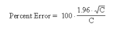
After counting a certain number of counts in your tube, you want to know what the "real" number of counts is. Obviously, there is no way to know that. But you can calculate a range of counts that is 95% certain to contain the true average value. So long as the number of counts, C, is greater than about 50 you can calculate the confidence interval using this approximate equation:

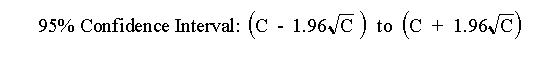
GraphPad StatMate (a program we shall use during the course) does this calculation for you using a more exact equation that can be used for any value of C. For example, if you measure 100 radioactive counts in an interval, you can be 95% sure that the true average number of counts ranges approximately between 80 and 120 (using the equation here) or more exactly between 81.37 and 121.61 (using StatMate).

When calculating the confidence interval, you must set C equal to the total number of counts you measured experimentally, not the number of counts per minute. Example: You placed a radioactive sample into a scintillation counter and counted for 10 min. The counter tells you that there were 225 cpm. What is the 95% confidence interval? Since you counted for 10 min, the instrument must have detected 2250 cpm. The 95% confidence interval of this number extends from 2157 to 2343. This is the confidence interval for the number of counts in 10 min, so the 95% confidence interval for the average number of cpm extends from 216 to 234. If you had attempted to calculate the confidence interval using the number 225 cpm rather than 2250 (actual counts detected), you would have calculated a wider (incorrect) interval.

The Poisson distribution explains why it is helpful to counts your samples longer when the number of counts is small. For example, this table shows the confidence interval for 100 cpm counted for various times. When you count for longer times, the confidence interval will be narrower.

Counting Time	1 minute	10 minutes	100 minutes
Counts per minute (cpm)	100	100	100
Total counts	100	1000	10000
95% CI (in counts)	81.4 to 121.6	938 to 1062	9804 to 10196
95% CI (in cpm)	81.4 to 121.6	93.8 to 106.2	98.0 to 102.0

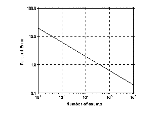
This graph shows percent error as a function of number of counts (C). Percent error is defined from the width of the confidence interval divided by the number of counts: