Home About SOP Admissions Academics Programs Activities Calendar of Events Resources Links Contact Us

3 Characterization of a Receptor Using a Radioligand Analysis of saturation radioligand binding data Saturation radioligand binding experiments measure specific radioligand binding at equilibrium at various concentrations of the radi-oligand. Analyze these data to determine receptor number and affinity. Because this kind of experiment used to be analyzed with Scatchard plots (more accurately attributed to Rosenthal), they are sometimes called "Scatchard experiments". The analyses depend on the assumption that you have allowed the incubation to proceed to equilibrium. This can take anywhere from a few minutes to many hours, depending on the ligand, receptor, temperature, and other experimental conditions. The lowest concentration of radioligand will take the longest to equilibrate. When testing equilibration time, therefore, use a low concentration of radioligand (perhaps 10-20% of the KD). Nonspecific binding (NSB) In addition to binding to the receptors, radioligand also binds to other sites termed nonspecific sites. Nonspecific binding is assessed by measuring radioligand binding in the presence of a saturating concentration of an unlabeled drug that binds to the receptor(s) of interest. The theory is that under those conditions, virtually all the receptors are occupied by the unlabeled drug, so the radioligand can only bind to nonspecific sites. Subtract the nonspecific binding at a particular concentration of radioligand from the total binding at that concentration to calculate the specific radioligand binding to receptors. [Discussion: what causes NSB and what can one do to minimize it.] Two questions should be obvious: 1) what unlabeled drug should you use, and 2) at what concentration? In characterizing an assay system, the rule of thumb is to use a different drug than the radioligand, ideally in a different chemical class. (Once a system is well characterized, it may be acceptable to use the same drug.) You want to use enough to block virtually all the specific radioligand binding, but not so much that you cause more general physical changes to the membrane that might alter specific binding. A useful rule-of-thumb is to use the unlabeled compound at a concentration equal to 100-1000 times its KD for the receptors. Nonspecific binding is usually linear with the concentration of radioligand (within the range it is used). Add twice as much radioligand, and you'll see twice as much nonspecific binding. 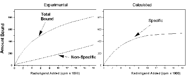The left figure shows a schematic of total and nonspecific binding. The figure on the right shows the difference between total and nonspecific binding, also known as the specific binding. If only a small fraction of the ligand binds to the receptor, then the free concentration of ligand equals the added concentration in both the tubes used to measure total binding and the tubes used to measure nonspecific binding. In this case, you can subtract the nonspecific from the total to get specific binding. If the assumption is not valid, then the free concentration of ligand will differ in the two sets of tubes. In this case subtracting the two values makes no sense, and determining specific binding is difficult, and other strategies are needed. 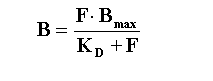Analysis of data to determine Bmax and KD As derived earlier, such experiments often are based on the One Site Binding Equation that we derived earlier: Again, this analysis is based on several assumptions: Only a small fraction of the radioligand binds. The free concentration is almost identical to the concentration you added. There is no cooperativity. Binding of a ligand to one binding site does not alter the affinity of another binding site. Your experiment has reached equilibrium. Binding is reversible and follows the law of mass action. Scatchard plots In the days before nonlinear regression programs were widely available, scientists transformed data into a linear form, and then analyzed the data by linear regression. There are a variety of algebraically equivalent ways to linearize such data, including the Lineweaver-Burk, Eadie-Hofstee, Wolff, and Scatchard-Rosenthal plots. With "perfect" data, all yield identical answers, yet each is affected more by different types of experimental error. The most commonly used of these methods in the pre-computer era was the Scatchard plot, where the X axis is specific binding (B) and the Y axis is specific binding divided by free radioligand concentration (B/F). 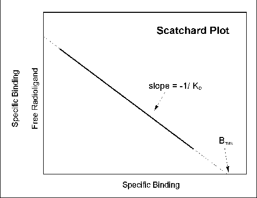It is possible to estimate the Bmax and KD from a Scatchard plot (Bmax is the X intercept; KD is the negative reciprocal of the slope). This transformation, however, distorts the experimental error, and thus violates the assumptions of linear regression. The Bmax and KD values you determine by linear regression of Scatchard transformed data are likely to be far from their true values. You should analyze your data with nonlinear regression. Do not analyze your data with Scatchard plots. After analyzing your data with nonlinear regression, however, it is often useful (traditional?) to display data as a Scatchard plot. The human retina and visual cortex are wired to detect edges (straight lines), not rectangular hyperbolas. Scatchard plots are often shown as insets to the saturation binding curves. They are especially useful when you want to show a change in Bmax or KD. When making a Scatchard plot, you have to choose what units you want to use for the Y axis. Some investigators express both free ligand and specific binding in cpm so the ratio bound/free is a unit-less fraction. While this is easy to interpret (it is the fraction of radioligand bound to receptors), a more rigorous alternative is to express specific binding in sites/cell or fmol/mg protein and the free radioligand concentration in nM. While this makes the Y axis hard to interpret visually, it provides correct units for the slope (which is -1/KD).